Grab a coffee and get comfortable; this is a long one! But I guarantee it is worth the read :) ~25min
Introduction
Shall we go all out for this project?
- Me and my project partner back in October 2025, a thought that made that October one of the most rigorous months ever.
This was the final project for EE2026 Digital Design. The course introduced students to fundamental digital design theories with practical applications using Verilog and an AMD Artix 7 FPGA.
Project ideas are open-ended as long as they fall within these constraints and meet these requirements:
- Only a single bitstream can be used.
- Must be within the resource limitations of the FPGA (which was 1800Kbits of BRAM and 90 DSP slices only!) A typical project would be 2D platform games (like Donkey Kong) or enhanced versions of the base graphical calculator using a Digilent PmodOLEDrgb of 96x64 pixel display.
However, fully open-ended projects are scarce, so we saw this as a golden opportunity to push the limits of what could be done with this introductory FPGA board.
We had two distinct goals in mind:
- The project should exploit the features of the FPGA: physical parallelism with low latency. In other words, it should not be something that could be easily done with a standard microcontroller or CPU (RTOS or OS threaded operations - virtual parallelism).
- It must be a product: a cohesively designed system that has a clear function, rather than a haphazard collection of disjoint functionalities.
Our Final Product and its Significance
Computer Vision. Specifically, an End-to-End Hardware-based Real-time Object Tracking System.
While FPGA-based vision systems exist in research, they are typically implemented on high-end boards with large memory resources. In contrast, this project was deliberately built under severe hardware constraints: a low-cost Basys3 FPGA, a teaching board with extremely limited on-chip memory and no external DRAM. We believed that this project will demonstrate the possibly unexplored capabilities of hardware-acceleration for computer vision.
Other than real-world applications of using FPGA for parallelised computer vision operations, we wanted the product to be interactive and fun.
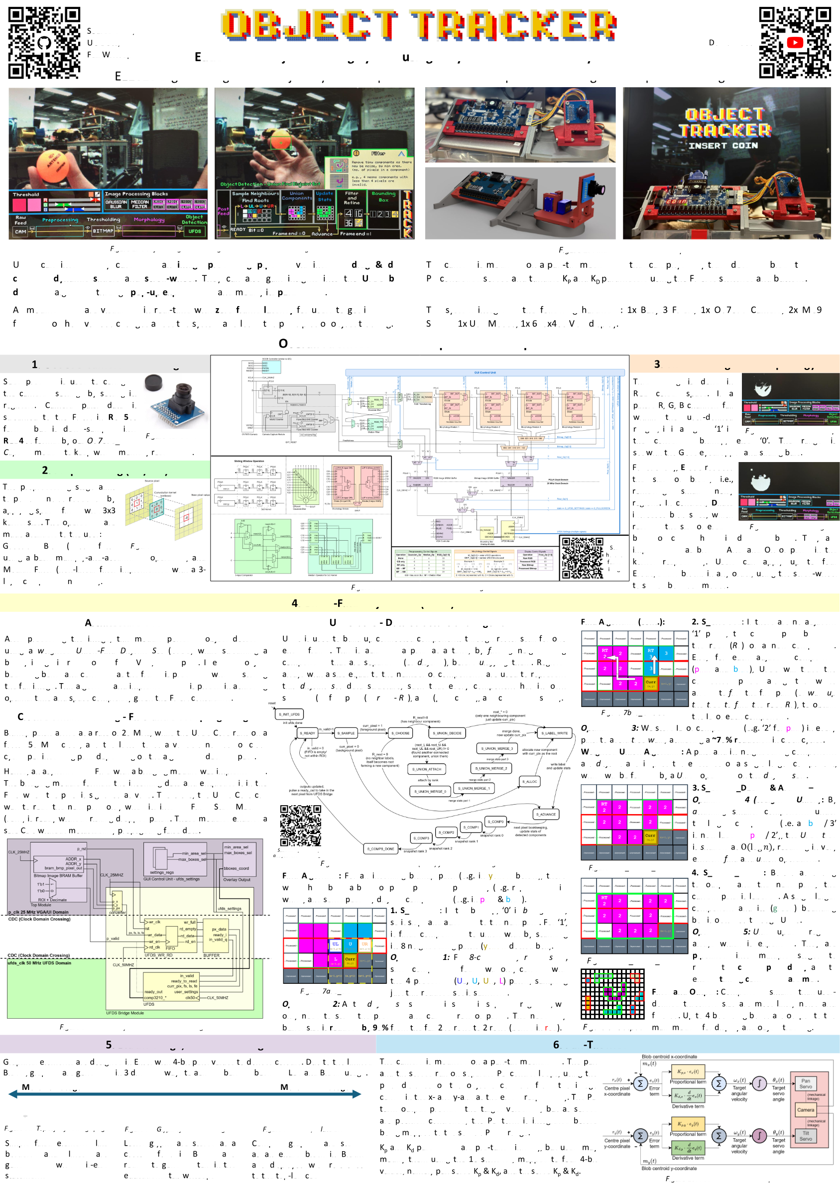
EE2026 FPGA Object Tracker Final Product
Ultimately, we settled to build an educational system to teach fundamental Computer Vision concepts. One where users can :
- interact through an intuitive GUI to customise an image processing pipeline via drag & drop controls, dynamic sliders and scroll-wheel
- gain insights into blob detection through our own algorithm using pop-up explanations and modifiable parameters.
- observe visual feedbacks on a monitor through VGA (instead of 96x64 pixels only)
- witness real-time object tracking by mounting the camera itself on a pan-tilt servo rig (with tunable PD controllers) that follows the detected object smoothly.
Our project met all of our desired outcomes: image processing and blob detection operations ran concurrently (physical parallelism) with fast, predictable memory access times to allow for real-time performance even with such limited hardware, while the GUI and pan-tilt assembly made for a fun and interactive product!
The sections after the demo video and poster detail the various components of the project and explains our design considerations made along the way, in a near chronological order of development.
Demo Video
Stay until the end of the video for fun section!
Poster
The poster is a concise, high-level overview of the system architecture and our design decisions.
If your browser blocks PDF embedding, open it directly here.
Here comes the details you have been waiting for!
The following sections go into much greater detail about the various components of the project, and our design considerations made along the way, in a near chronological order of development.
Feel free to use the table of contents on the left to navigate to specific sections as well!
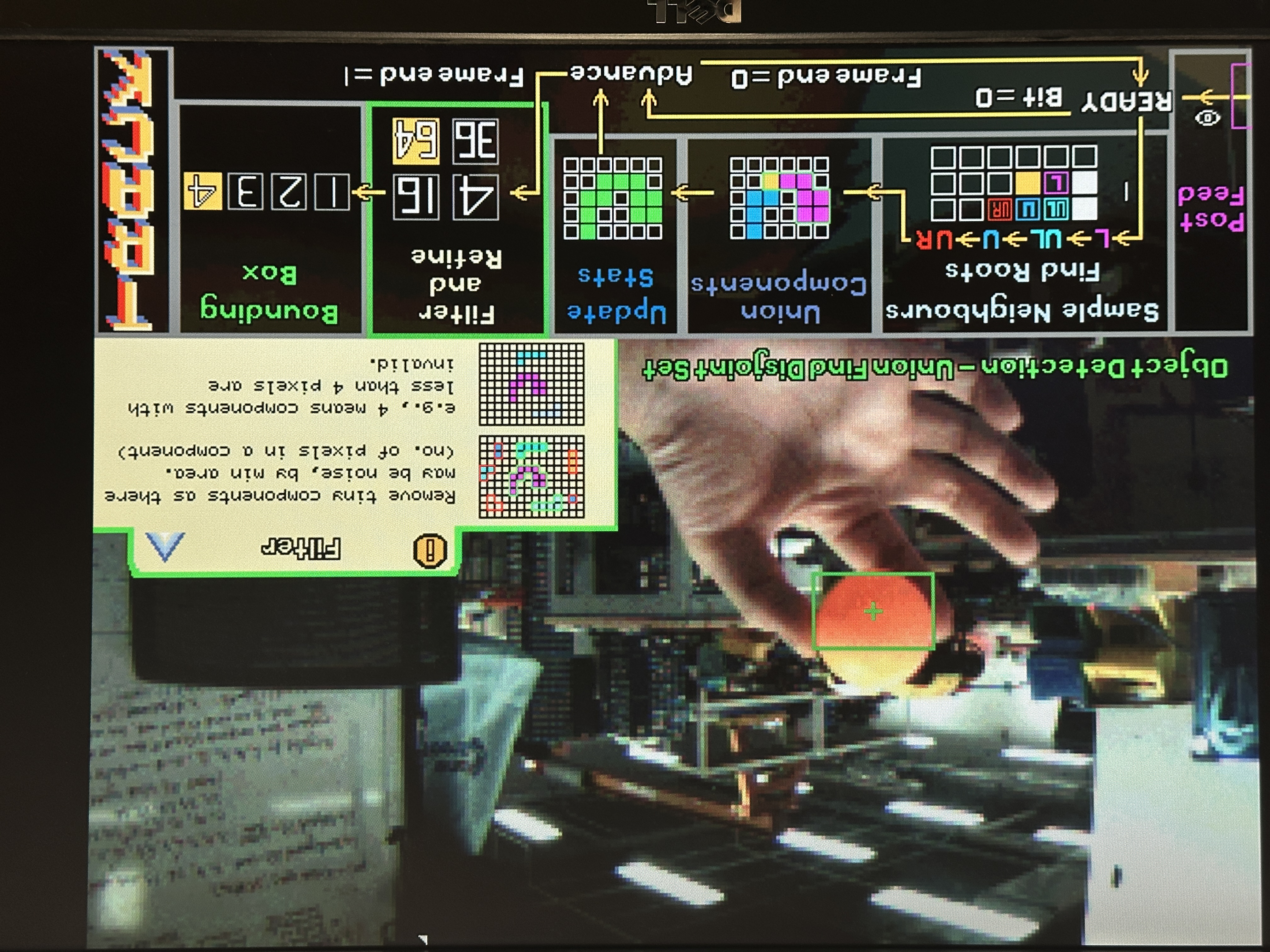
CV Pipeline
The overall architecture of the CV pipeline is shown in the diagram below. Broadly speaking, the pipeline can be divided into 5 main stages:
- Camera Interfacing (Grey): Configuring the camera’s settings and capturing pixel data from camera capture.
- Pre-Processing (Green): Blurring the image to reduce noise using spatial filters (Gaussian Blur or/and Median Filter) through convolusion kernel techniques.
- Thresholding and Morphology (Orange): Thresholding the image based on user-defined colour ranges to create a binary bitmask, which undergo Erode/Dilate operations to clean up noise.
- Blob Detection (Yellow): Searching contiguous regions in the bitmask and compute centroids/bounding boxes using *Union-Find Disjoint Set (UFDS) *i.e. finding objects.
- Buffering and Display (Purple): Saving the processed image into BRAM buffers and rendering them on the VGA display.
In addition, user settings from the GUI (Blue) are decoded into control signals that modify the datapath accordingly, as summarised in the tables at the bottom.
Overall CV Pipeline Diagram
Image Processing
Data preparation is the first crucial step of a computer vision workflow.
This includes:
- Data collection by gathering raw data from the camera
- Data pre-processing which formats gathered data into a suitable form and cleans up noise (or unwanted data) before piping them into our detection algorithm.
OV7670 Camera Interfacing
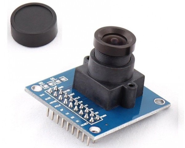
OV7670 Camera Module
The OV7670 camera is connected to the Pmod pins of the FPGA. Its settings is first configured by setting its registers over SCCB protocol (an I2C-like register-write protocol). Camera pixel data is then streamed to the FPGA as RGB565 byte-pairs on the camera’s PCLK with VSYNC/HREF framing.
Keeping Basys3 BRAM limits in mind, we have to avoid buffering a full 640×480 RGB565 frame (4,915,200 bits per frame!). Hence, our OV7670_Capture down samples each pixel to RGB444 format, and decimates into a 310×240 Region of Interest (ROI) by writing into BRAM only on even coordinates, resulting in 892,800 bits per frame.
Memory Optimsisation and Tradeoff with Resolution
This tradeoff between resolution and memory is strategic as the reduction in resolution was barely affecting performance, but it significantly reduced our memory usage for frame capture by ~80%!
We have completed our data collection.
Pre-Processing (Gaussian Blur and Median Filter)
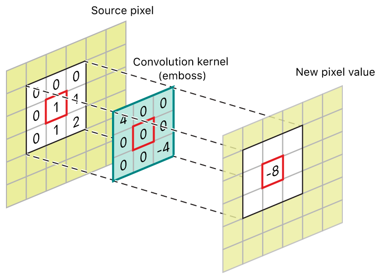
Convolution and Sliding Window Visualisation
TODO: insert gaussian blur and median filter visualisation, and noise from raw capture
The first data pre-processing step is to eliminate noise from our raw capture. This is done through two spatial filters:
- Gaussian Blur: a linear filter using multiply-and-accumulate operation on a fixed kernel
- Median Filter: a non-linear filter implemented with a 3-layer comparator network; applied per-channel on RGB444
All image ops run one-pixel-per-cycle using a 3×3 sliding window.
TODO: complete this summarised writeup.
Thresholding and Morphology (Erode/Dilate)
The idea of object detection through colour is blob detection. To generate the desired blobs, two additional data pre-processing steps are required: thresholding and morphology filtering.
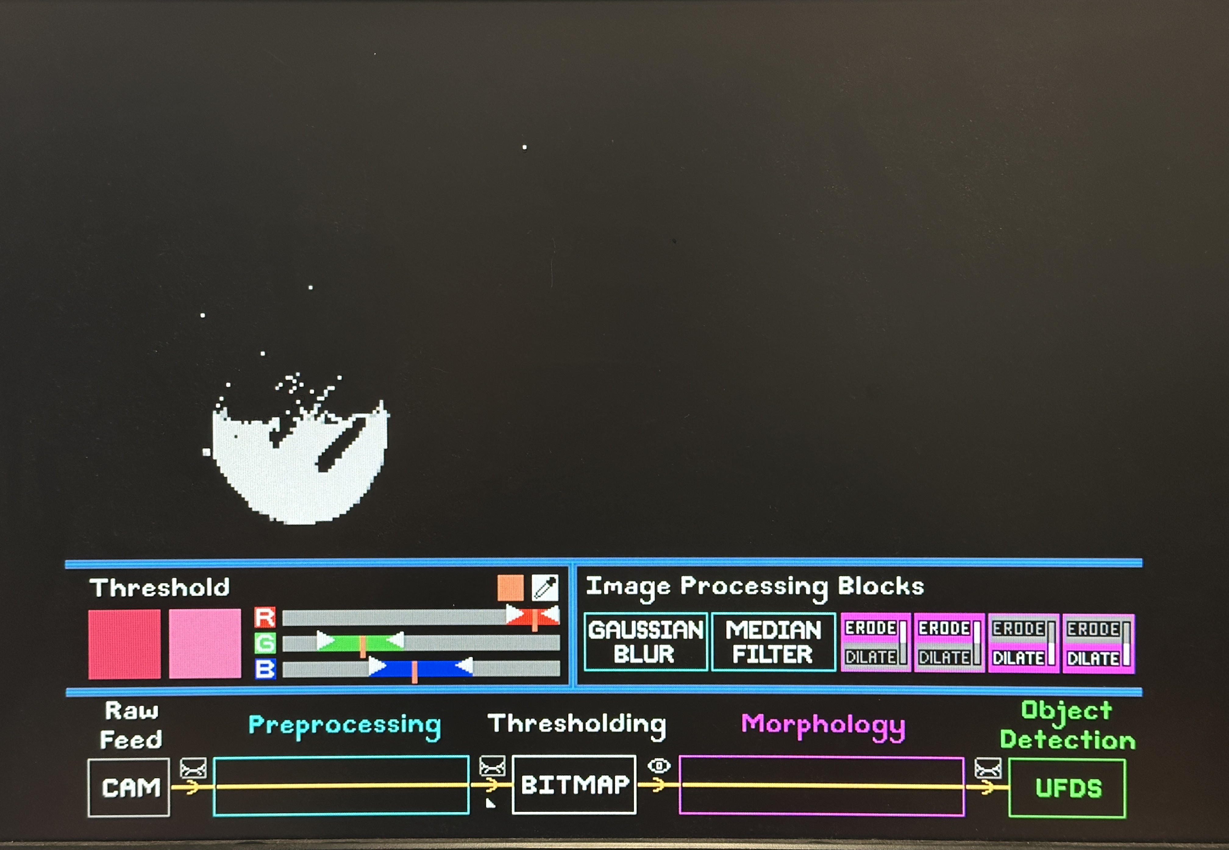
Thresholding is done in RGB colour space, which formats our data from RGB to a 1-bit bitmap for our detection algorithm. Using an eyedropper, users select a specific colour from the object. They then define the upper and lower bounds of Red, Green and Blue channels using sliders on our GUI. These bounds are piped into our thresholding module, such that if a pixel’s R, G, B channels fall within the user-defined ranges, it is assigned 1 in the converted bitmap, else 0.
Better representation of colour space
Given more time, other colour spaces such as HSV would have been a more intuitive representation of the image, especially when it comes to thresholding. The ideal thresholding step would be through a visualisation of the colour range for users to choose. However, the concept of a range in RGB space is hard to represent and visualise, as compared to a range using hue, saturation and (TODO: what is V?), either through colour histogram or HSV cylinder. Due to time constraints, we carried on with RGB, but mitigated by implementing an eye dropper feature that instantly draws 3 vertical markers on the R, G, B sliders, and users may change to bitmap view to tune the range of each slider to obtain a reasonably sized blob.
As seen from the previous bitmap picture, the “blob” that is supposed to represent the ball object is fragmented into many bits, and there are “noisy” or unwanted bits that fell within the user defined range. This is where Morphology Filtering is needed: to clean up the bitmap.
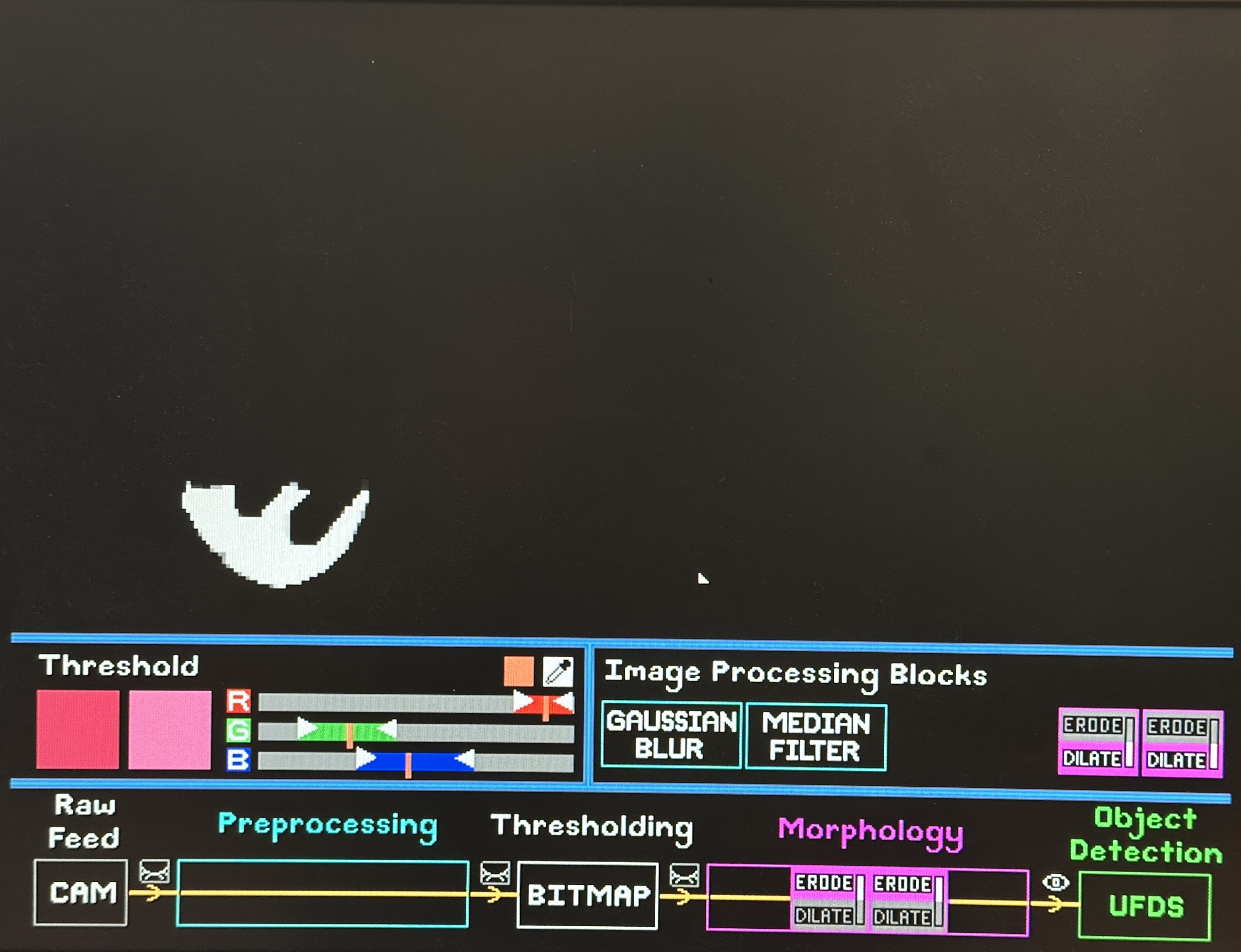
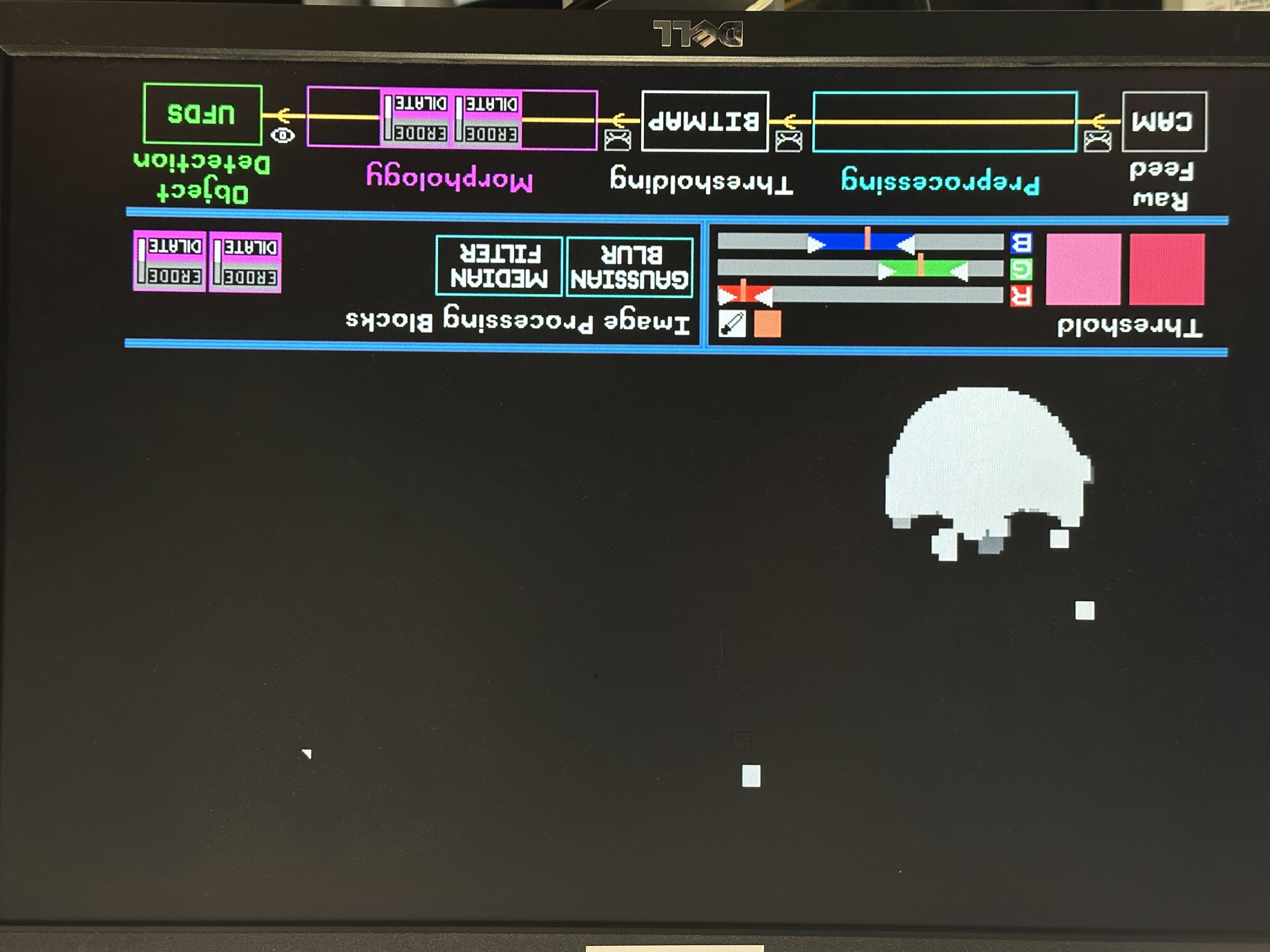
We strategically reuse the same 3x3 convolution kernal sliding window trick used in Gaussian Blur and Median Filter for our Morphology blocks. The difference lies in the operations executed:
- Erode: reduces the size of blobs, i.e., removing small noisy regions. Logical operation: bitwise AND of pixels in kernel.
- Dilate: increases blob sizes, which restores the size of eroded blobs or covers holes in detected blobs. Logical operation: bitwise OR of pixels in the kernel.
Users can apply up to four Erode/Dilate blocks in any order, using the scroll-wheel to switch between modes, until a bitmap with nicely unified blob(s) of little noise is achieved for blob detection
More details on Image Processing
This section is explained in much greater detail by my teammate here.
This write up is still work-in-progress. You may proceed but it is unrefined…watch the demo video and read the poster in the meantime!
If you have any questions, feel free to reach out to me :)
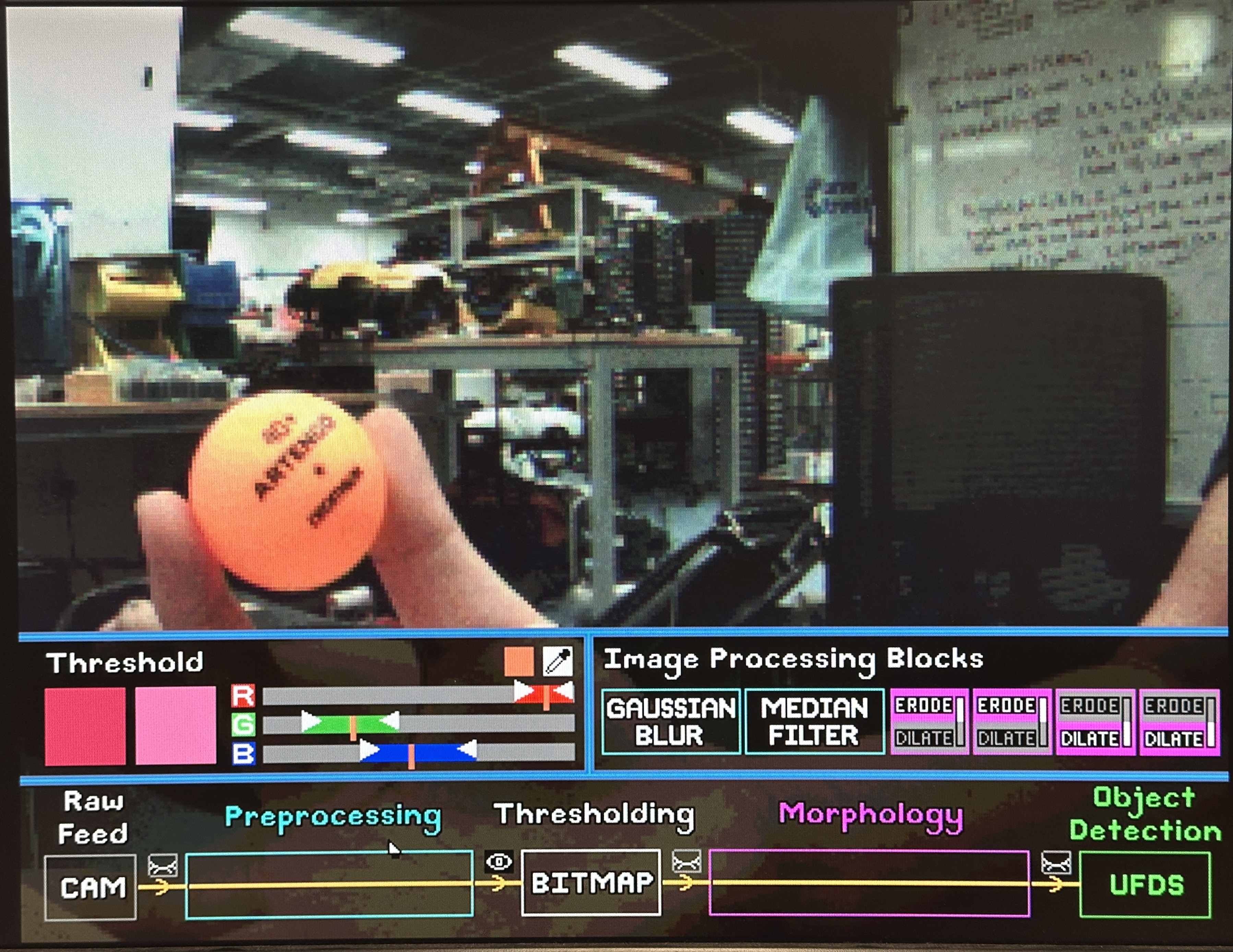
Complete Implementation of Union-Find Disjoint Set (UFDS) Algorithm in Verilog for Blob Detection
This section presents the detailed implementations of every step, decisions and personal thoughts, failures, iterations and testings. Here are two pictures and a video of the blob detection at work!
TODO: insert video?
Architecture Overview
After processing the image, this module performs object detection using a weighted Union-Find Disjoint Set (UFDS) while streaming a binary image in raster order from VGA/BRAM path. It extracts object bounding boxes and centroids as the frame is processed without storing the full image. This algorithm and implementation is pivotal in achieving optimal time and space complexity given the FPGA constraints.
The blob detector is a streaming connected-components labeling engine implemented as a union-find data structure that operates directly on the thresholded/morphed bitmap. The core idea is to scan pixels in raster order and assign labels to foreground pixels while maintaining equivalence classes between labels that later turn out to be connected. Instead of storing the whole image, the design maintains only the minimum state required for correctness: a small neighborhood context (the reduced neighbor set for connectivity), per-label parent/rank arrays, and per-label statistics required to emit bounding boxes.
In the top-level integration, UFDS does not see the full 640×480 scan; it sees the 310×240 ROI stream at a decimated rate. Top explicitly gates the UFDS feed with in_roi and a decimation condition (decim_hv) so that, despite double-scanned VGA output, UFDS receives exactly one sample per ROI pixel. This gating is critical because union-find assumes a consistent raster progression; if pixels are duplicated due to display scaling, the component statistics and bounding boxes would be wrong.
Cross Domain Crossing (CDC) Solution for UFDS Algorithm
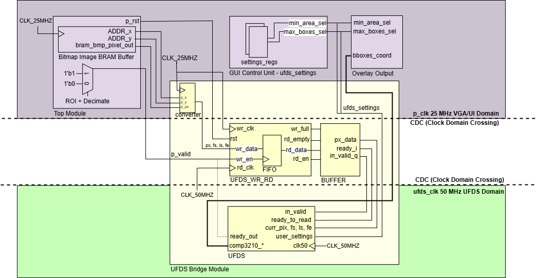
Clock Domain Crossing for UFDS
The UFDS blob detector is intentionally clocked faster than the VGA domain because its per-pixel work is not constant-time. Even though pixels arrive in raster order at clk25, the union-find core runs at clk50 and may spend multiple cycles per pixel performing find/union operations, updating statistics arrays, and handling state transitions. That mismatch creates a classic producer–consumer problem: the VGA domain can produce pixels at a fixed cadence, but the UFDS domain consumes pixels at a variable cadence.
This is solved with a two-part CDC architecture: an asynchronous FIFO (UFDS_FIFO) for safe clock-domain crossing, and a “ready/valid bridge” (UFDS_Bridge) that adds backpressure so the UFDS FSM is never forced to accept a new pixel before it is ready. On the producer side (VGA domain), the stream is packed into a small word containing {frame_start, line_start, frame_end, pixel} so UFDS can reconstruct raster context without needing external counters. Writes occur whenever the pixel is valid within the ROI. The FIFO itself uses dual-clock memory with Gray-coded read/write pointers and synchronized pointer transfer, which is the standard technique to avoid metastability when checking full/empty across domains.
On the consumer side (UFDS domain), UFDS_Bridge does not simply “read whenever FIFO is non-empty”. Instead it maintains a one-word staging buffer and only asserts in_valid when the UFDS core asserts ready_to_read. This detail is important: it transforms the asynchronous FIFO into a clean decoupled interface where the UFDS FSM can throttle input at pixel granularity, guaranteeing that union-find work is never corrupted by dropped or duplicated pixels. In other words, the FIFO handles clock correctness, while the bridge handles protocol correctness for a variable-latency algorithm.
A fundamental understanding of UFDS
Union-find (disjoint set) represents a partitioning of elements into sets using a parent-pointer forest. Each element points to a parent; roots are elements that point to themselves and represent an entire set. The two core operations are find(x), which returns the root of x’s set (often with path compression), and union(a, b), which merges two sets by attaching one root under the other (often by rank/size). In connected-components labeling, each provisional label corresponds to an element, and unions are performed when the current pixel is connected to already-labeled neighbors.
In hardware, the “elements” are not pixels; they are labels allocated during the scan. That distinction matters because it bounds memory usage: instead of storing per-pixel labels for the full frame, we store per-label metadata and only keep enough row history to know which label is above/upper-left/upper-right of the current pixel.
Disjoint Set Representaion in FPGA Registers
In UFDS_Detector (inside UFDS.v), disjoint-set state is implemented as BRAM-style register arrays for parent[] and rank[], alongside statistics arrays that accumulate component properties as the scan proceeds. Typical statistics include area (pixel count), centroid sums (to compute cx/cy), and min/max extents (left/right/top/bottom) for bounding-box emission. Because union operations can merge two previously separate components, the implementation must be careful about where statistics “live”: when two roots are merged, one root becomes the canonical representative, and the statistics must be merged into that representative so future pixels update the correct component.
To support a streaming scan without full-frame label storage, the detector maintains a two-row labeling buffer and a reduced neighbor set. At each pixel, it evaluates connectivity to a small set of already-visited neighbors (typically left, upper-left, up, and upper-right). This is sufficient for 8-connectivity when scanning left-to-right, top-to-bottom, and it avoids needing to look ahead into unvisited pixels.
The Full Finite State Machine (FSM)
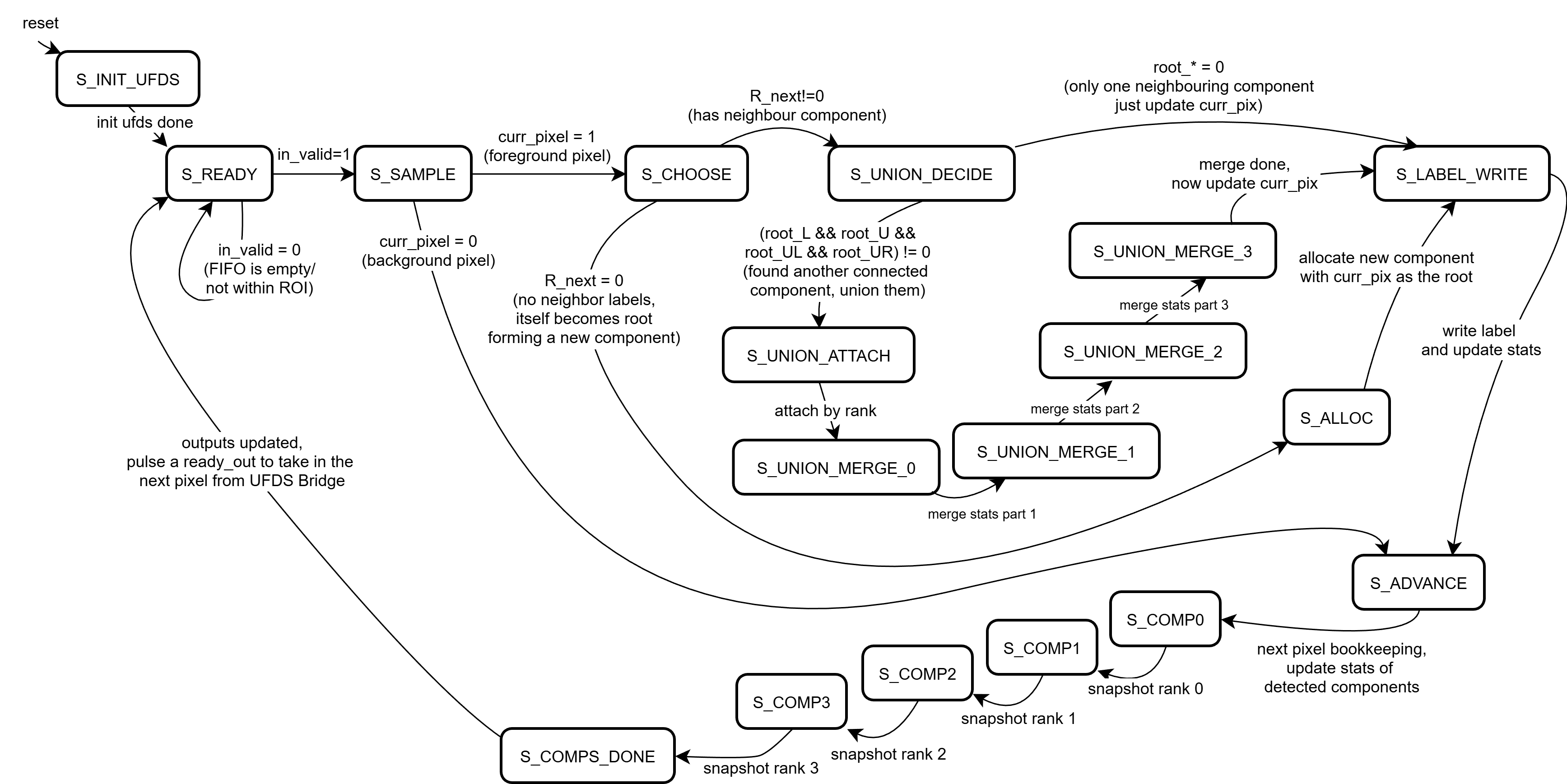
The UFDS Finite State Machine Diagram
The union-find engine is explicitly written as a finite state machine because find and union are not combinationally cheap. A find operation is a pointer-chasing loop over parent[] until a root is reached, and union must compare ranks, attach one root to another, and merge statistics deterministically. Implementing these steps as a multi-state FSM at clk50 keeps timing closure feasible on a Basys3-class device while still allowing the system to sustain a real-time frame rate.
At a high level, the FSM alternates between (1) sampling the next pixel and its neighbor labels, (2) choosing an action (new label, reuse a neighbor label, or union two labels), (3) executing the necessary find/union steps, and (4) updating per-component statistics before advancing the raster position. The key control signal that makes this composable with the CDC bridge is ready_to_read: the UFDS core asserts readiness only when it is safe to accept the next packed pixel token. This makes “one pixel equals one iteration” a protocol, even if that iteration takes multiple cycles internally.
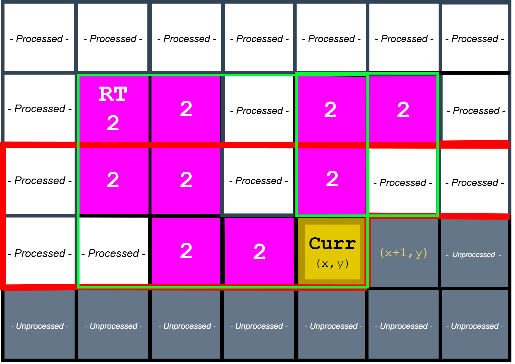
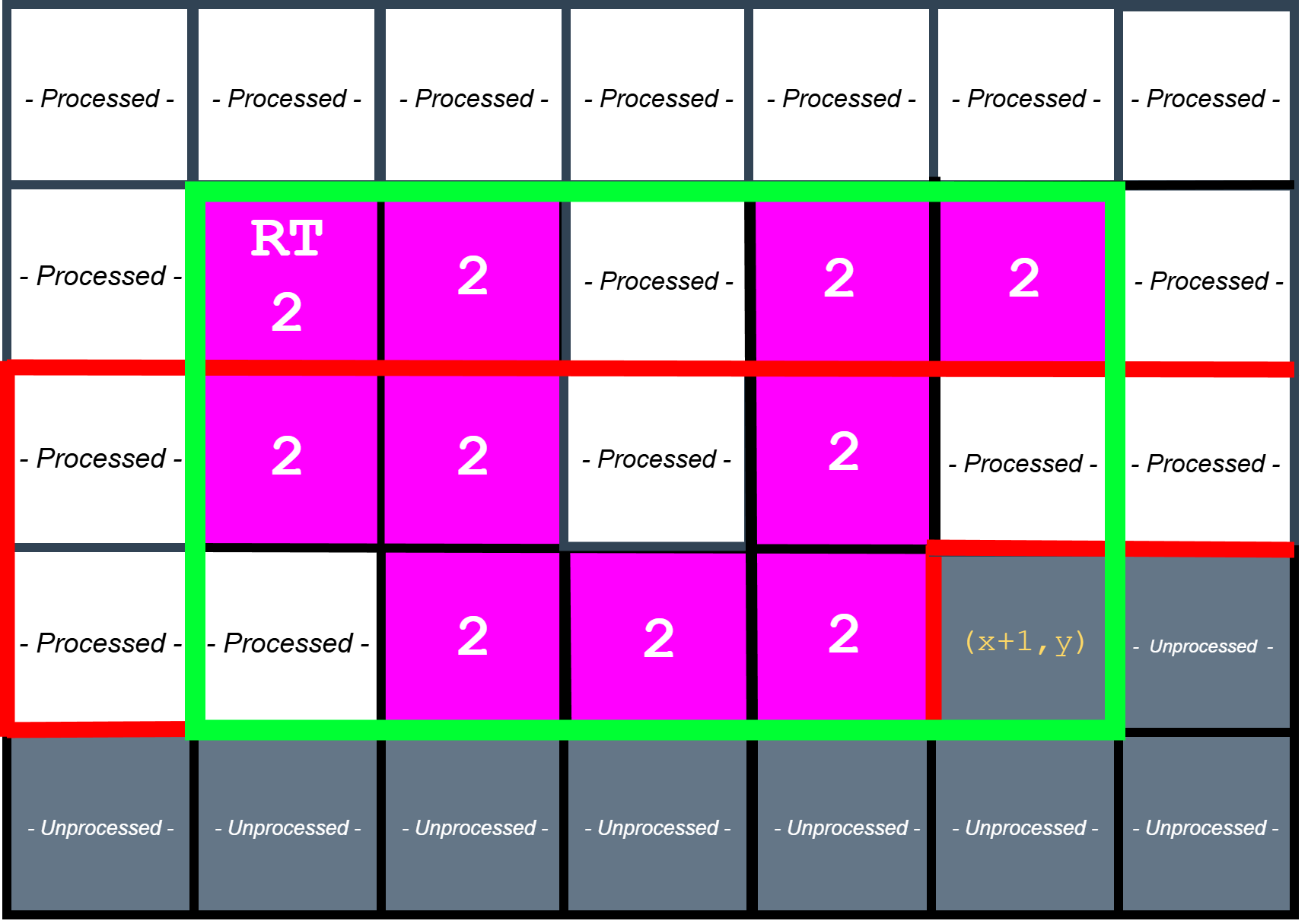
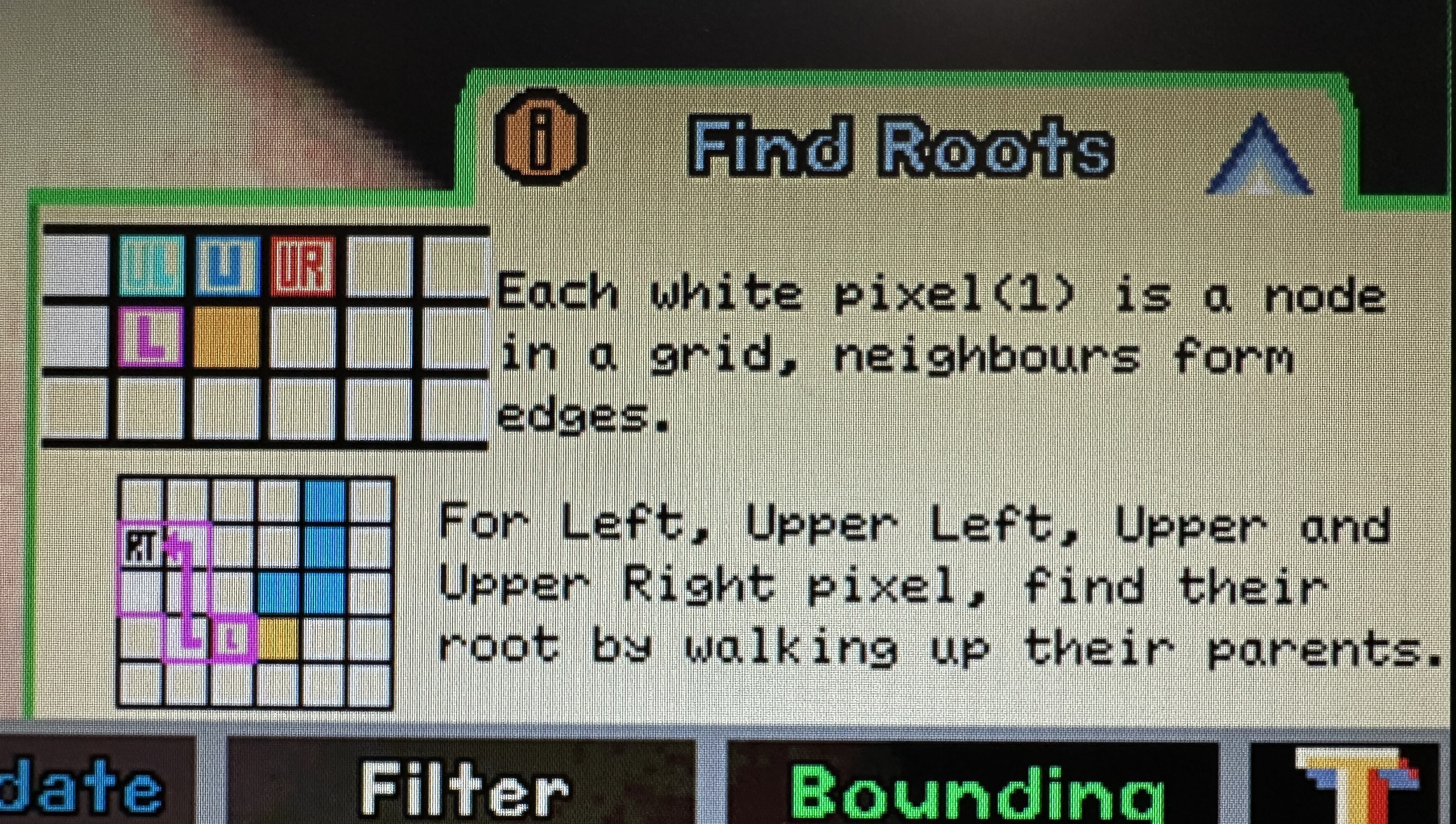
Sample neighbours
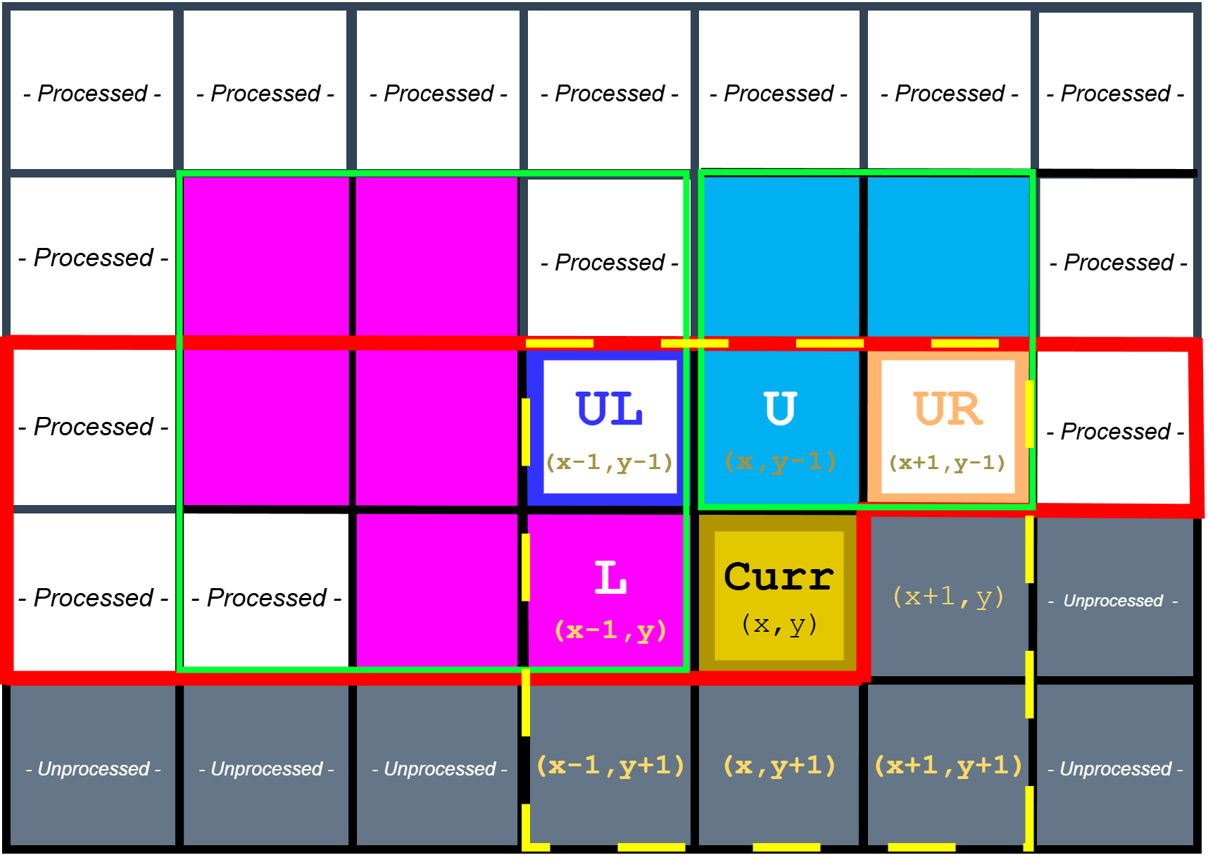
Sampling reduced neighbourhood set of pixels for 8-connectivity raster scan
For each foreground pixel, the detector samples the reduced neighbor set (labels from the previous row and the current row’s left neighbor). If no neighbor is labeled, a fresh label is allocated and installed into the current position in the row buffer. If exactly one neighbor label exists, that label is propagated to the current pixel and its statistics are updated (area increments, centroid sum accumulates, bounding extents are expanded if needed). When multiple neighbor labels exist and disagree, the current pixel becomes the “witness” that those labels are equivalent, and the FSM schedules a union operation.
Find Operation
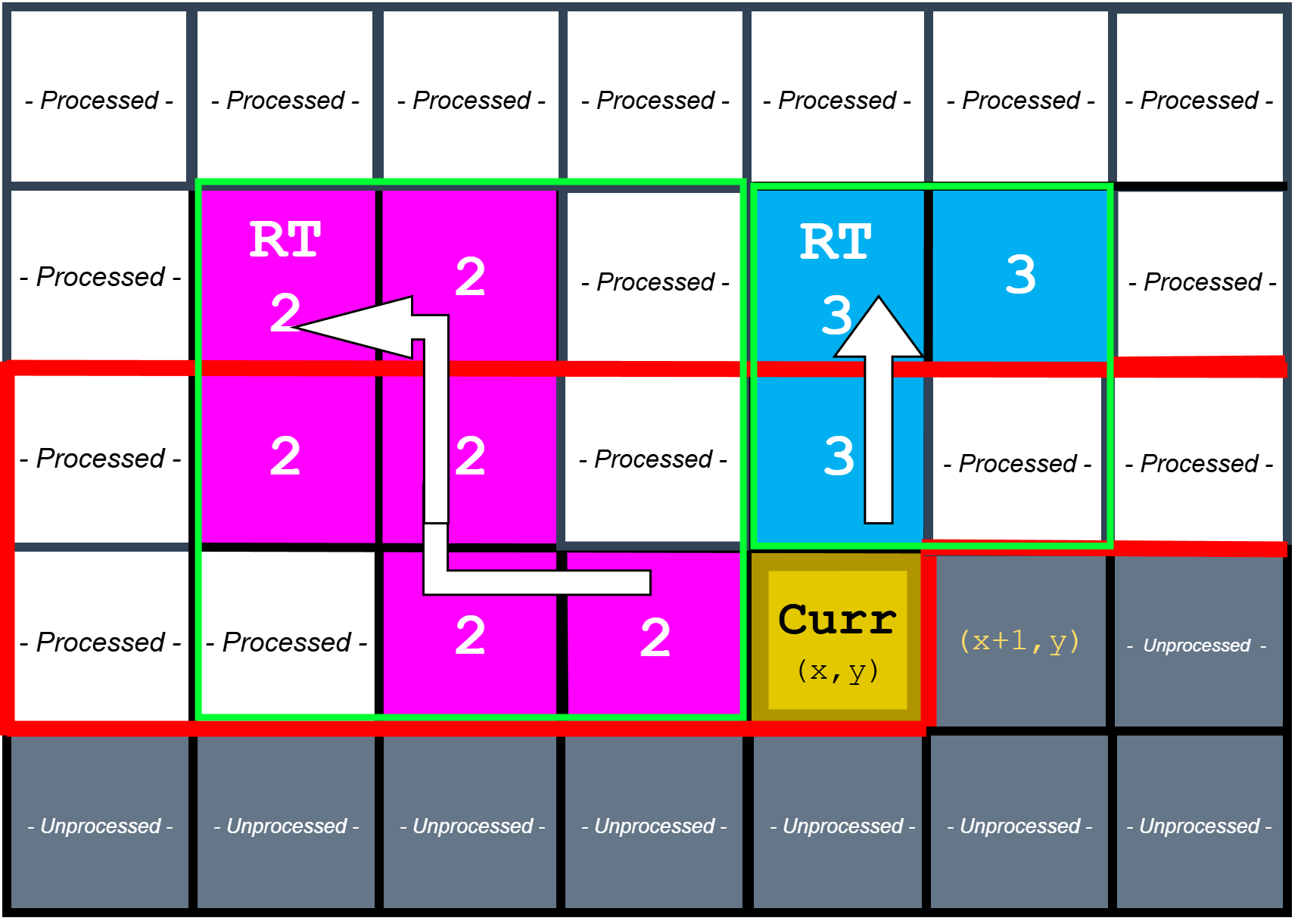
Find operation to identify roots of neighbouring components
The find operation is implemented as iterative traversal of the parent[] forest until a root is found. Because this traversal can take multiple steps (especially early in a frame before unions have stabilized), it is naturally expressed as a sequence of FSM states rather than a single-cycle combinational loop. This is also where the CDC bridge becomes essential: the UFDS core must be allowed to stall input consumption while it resolves roots, otherwise the raster input stream would outrun the label resolution logic.
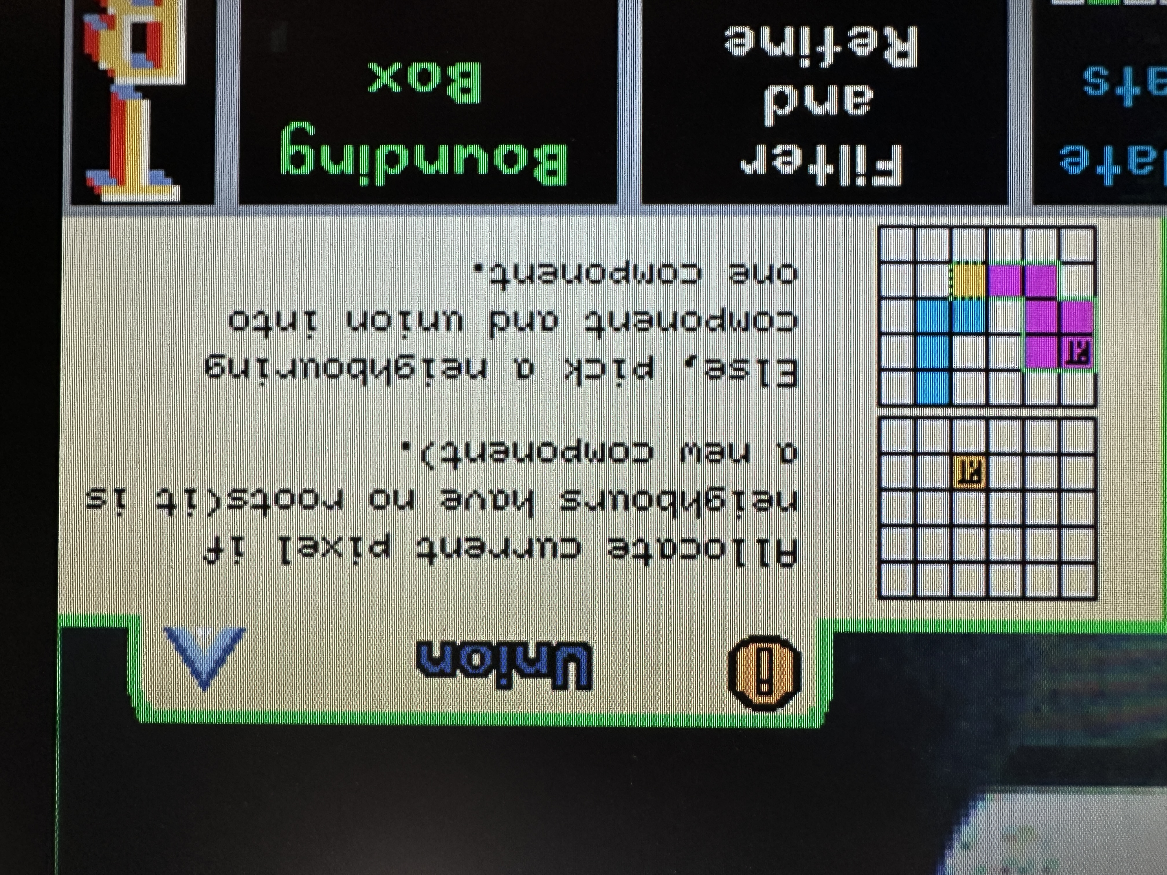
Weighted Union Operation
Weighted union operation to merge component roots
When two roots must be merged, the design performs a weighted union (by rank) so the parent tree remains shallow, reducing the average cost of subsequent finds. The chosen root becomes the canonical component, and the losing root’s statistics are folded into it. This is also the point where bounding box and centroid calculations become meaningful: by continuously merging stats into the canonical root, the detector ensures that the final output for a component is correct even if its equivalence class was discovered gradually across the scan.
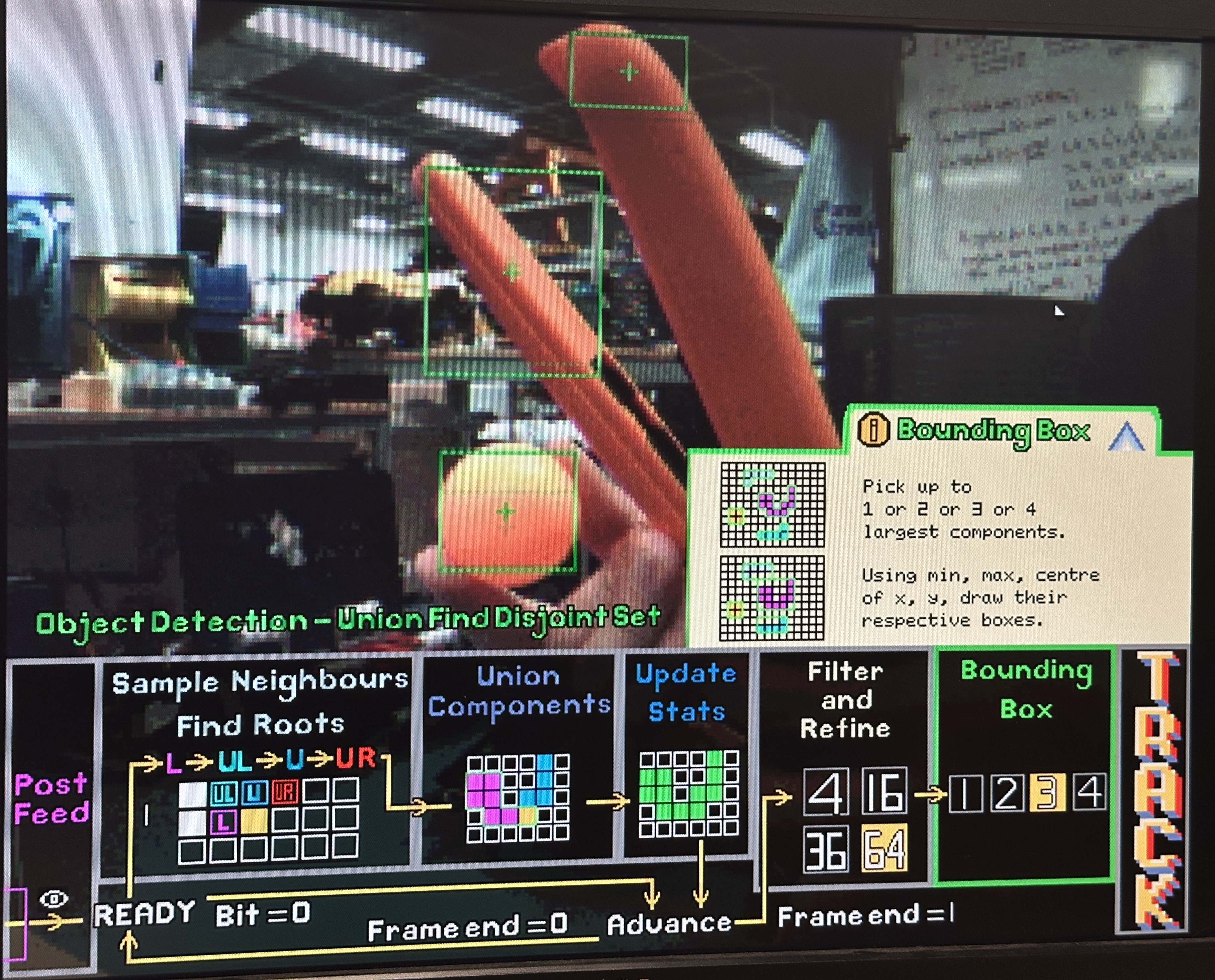
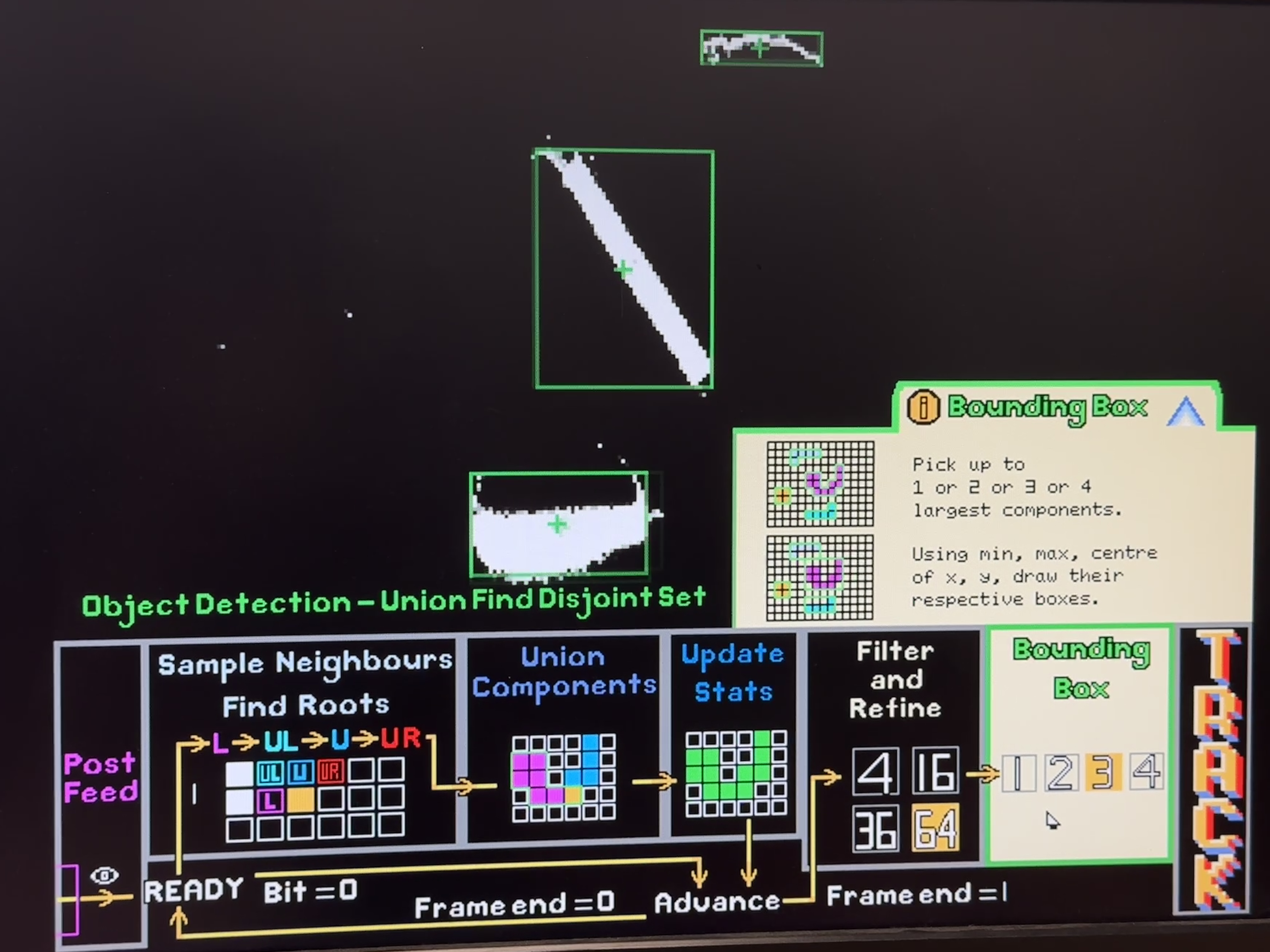
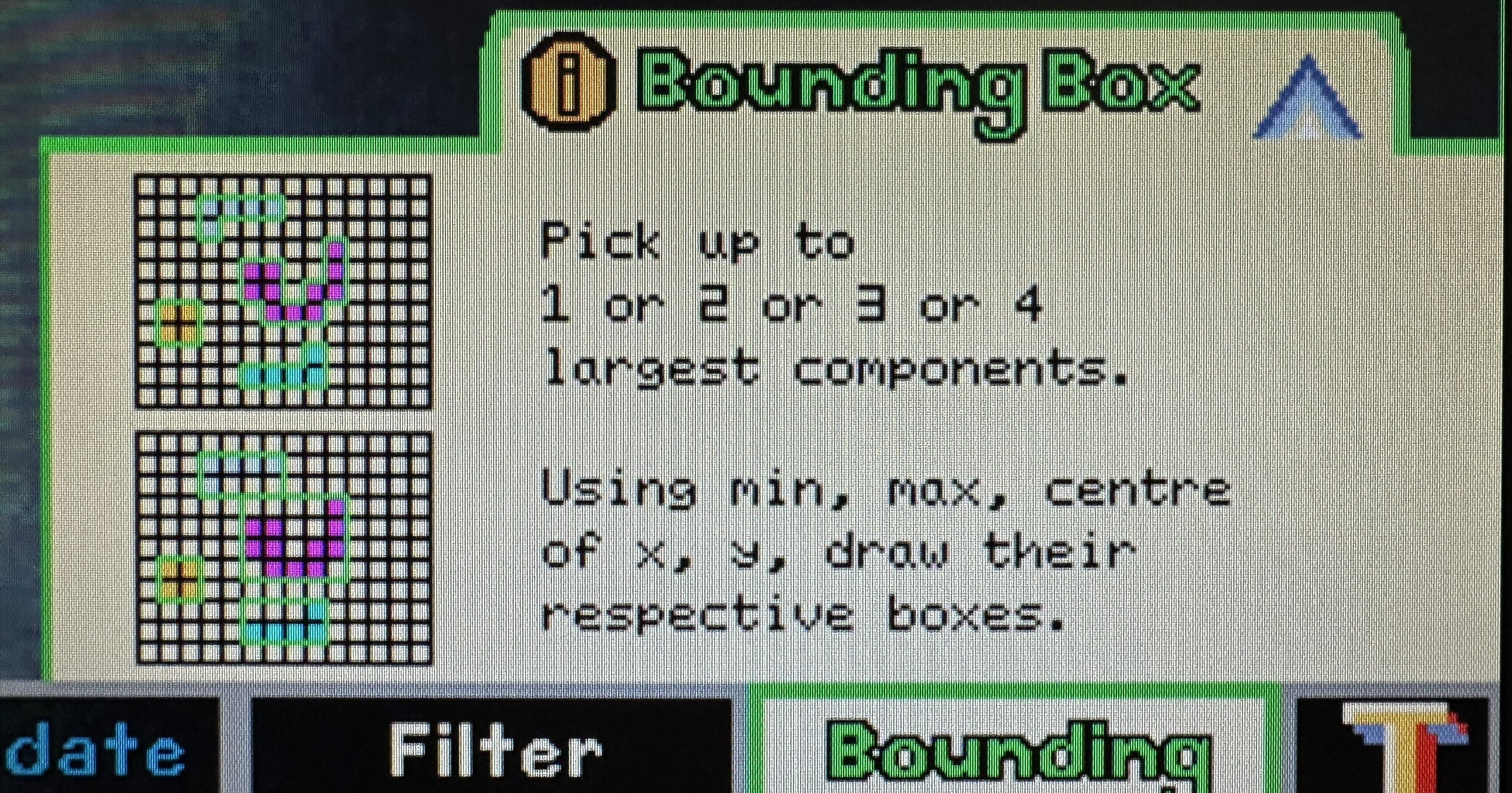
Updating Statistics and Emitting Bounding Boxes
Updating statistics and emitting bounding boxes
After labeling/unioning a pixel, the FSM updates the relevant component statistics. For area and centroid sums, this is a simple increment/addition. For bounding boxes, the FSM compares the current pixel’s coordinates against the component’s recorded extents and updates left, right, top, and bottom as needed. At frame end, the detector iterates over all allocated labels, identifies roots, and emits bounding boxes for components that meet the minimum area threshold.
Testings and Simulations
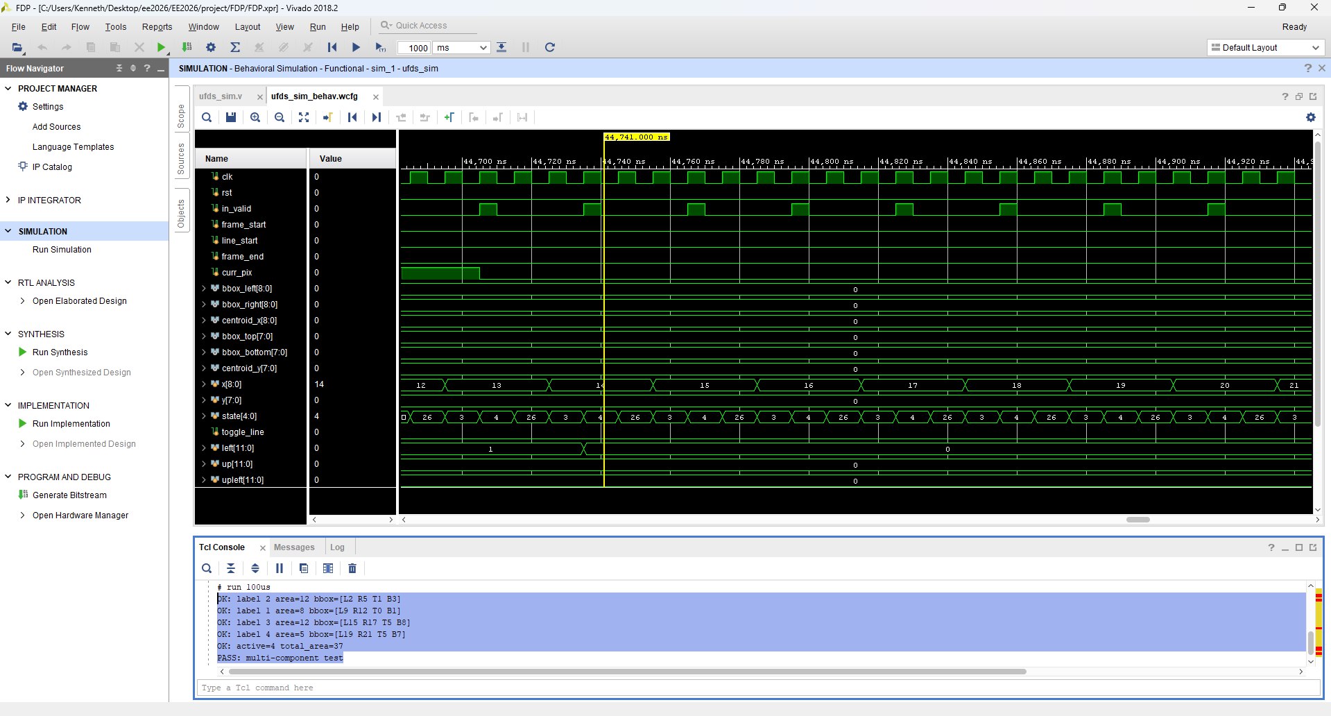
Simulation using small test frame
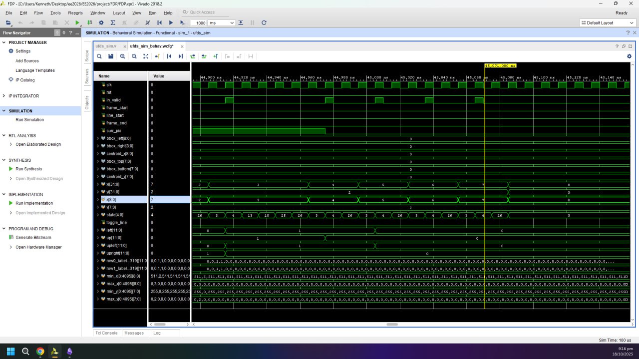
Full Simulation showing all internal signals
Because this is a live video system, a large part of validation is performed in situ using the on-screen instrumentation. UFDS outputs are latched once per VGA frame (so bounding boxes do not “tear” mid-frame) and then rendered back onto the ROI using explicit coordinate comparisons. This makes correctness observable without a software debugger: if unions are wrong, components fracture; if neighbor sampling is wrong, bounding boxes drift; if CDC is wrong, the overlay becomes unstable or visibly inconsistent. In addition, the UFDS settings UI includes an educational tab system that visualizes the algorithm’s stages, which doubles as a sanity-check that the internal conceptual model matches the actual FSM behavior.
Graphical User Interface (GUI) Design in Verilog
The GUI is implemented as a composited overlay in the VGA clock domain, split into two rendering mechanisms depending on the type of graphic. For crisp geometric primitives (borders, separators, toggle hitboxes), the design uses combinational pixel generators such as cv_settings_overlay and ufds_settings_overlay that compute overlay_en/overlay_rgb directly from (px, py) and the current UI state. For more complex artwork (icons, labels, and the educational tab bitmaps), the design uses BRAM-backed sprites via generate_bram_overlay, which turns on-screen coordinates into a BRAM address (overlay_addr) and fetches a compact indexed pixel value from overlay_mem.
The BRAM overlay pipeline is timing-aware. generate_bram_overlay computes frame_x_next/frame_y_next and intentionally “looks ahead” by multiple pixels, because BRAM reads have a multi-cycle latency; the module even advances x by 3 per decision to align with the 2-cycle delay. Without this lookahead, the fetched sprite pixel would be spatially shifted relative to the raster position. This is one of those hardware-specific details that you rarely think about in software UI work: the framebuffer is not a random-access surface; it is a stream, so even drawing text is a synchronous pipeline problem.
Educational Tabs
The educational tabs are primarily implemented in the UFDS settings page. ufds_settings_overlay maintains an internal tab_idx that selects which stage of the algorithm is being explained (sample/find, union, update stats, filter, draw bounding boxes). Clicking a tab is pure hit-testing in VGA coordinates on left_edge, and the selection is latched so the content is stable across frames. The overlay also produces an info_dim_en mask, which Top uses to dim the live camera feed under the info panel while keeping the rest of the frame readable.
The tab content itself is drawn using BRAM sprites. generate_bram_overlay uses info_idx to select which educational images to place inside the panel, and it computes sprite addresses relative to an (ufds_t_x, ufds_t_y) origin so the entire tab block can slide/animate as a single unit. This arrangement keeps the overlay logic simple: the “what to draw” decision stays in the control plane (tab_idx/info_idx), while the “how to draw it” stays in the dataplane (BRAM lookups with correct latency alignment).
Drag and Drop
Drag-and-drop is implemented as a deterministic state machine in cv_settings_dragdrop operating entirely in VGA coordinates. The module defines six movable boxes (Gaussian, median, and four morphology blocks), computes per-box hover flags (hov0..hov5), and starts a drag on a debounced press edge (mouse_left_edge). While dragging, the selected box’s top-left position is continuously updated so that the cursor remains centered on the box, with explicit clamping to the 640×480 screen bounds.
Releasing a drag is intentionally filtered to avoid accidental drops due to noisy button transitions. Instead of relying purely on a falling edge, the design requires the left button to be continuously low for DRAG_RELEASE_TH cycles (2,000,000 cycles at 25 MHz, roughly 80 ms) before treating it as a drop. Once dropped, the module checks whether the center of the box lies within the correct drop zone, which prevents edge-cases where only a corner overlaps. If the placement is invalid, the box snaps back to its original home position and its placed*_pre/placed*_morph flag is cleared.
Bin checks for Morphology Boxes
In hardware, “bin checking” is just geometry and classification, and the design makes this explicit. Each morphology box has an in-drop test (in_m2..in_m5) against the morphology drop zone, and placement is captured by placed2_morph..placed5_morph. The type of each morphology block is also dynamic: the box is not permanently “erode” or “dilate”. Instead, each box holds an is_erodeX flag, which can be toggled by the scroll wheel while hovering. This means the UI exposes both structural configuration (which boxes are placed, and in what order) and semantic configuration (whether each placed step behaves as erosion or dilation).
The outputs of this system are purpose-built for downstream RTL consumption. The module exports a compact morph_vector (one bit per stage indicating dilation) and a box_morph_vector (the per-box type flags), and it also exports a box_order_vector that encodes which physical box currently occupies each left-to-right slot. That encoding makes it easy for the datapath to drive the four instantiated Morphology_3x3 blocks without needing complex per-box metadata.
Snapping in Place
Snapping is designed to be visually consistent and logically meaningful. For preprocessing, the drop zone supports up to two blocks, and cv_settings_dragdrop computes a centered layout: one block is centered, while two blocks are centered as a pair with fixed spacing. For morphology, snapping supports up to four blocks, and the layout is computed from a left-to-right rank (r2..r5) that counts how many other placed morphology blocks are strictly to the left. Based on the placed count, the module computes a left margin (morph_left_margin_N = (morph_w - N*W_MOR)/2) and assigns snapped positions as morph_x + margin + W_MOR * rank. This produces a clean “pipeline” look and ensures that the left-to-right spatial order is exactly the logical processing order.
Scroll Wheel
The scroll wheel is a small interaction, but it is implemented in a way that stays faithful to synchronous design. While not dragging, scroll pulses (scroll_up / scroll_down) are interpreted only when the cursor is hovering over a morphology box, and the corresponding is_erodeX flag is toggled. That flag then influences both the recorded morphology order codes and the BRAM overlay sprite selection, so the UI and the underlying control vector remain consistent.
Overall Data Path
At the system level, the design is a three-domain pipeline: the camera capture domain (ov7670_pclk) writes decimated ROI pixels into BRAM, the VGA domain (clk25) reads and composites the selected “final” view (raw, preprocessed, bitmap, or morphology) while servicing all GUI hit-testing and overlay drawing, and the UFDS compute domain (clk50) consumes the binary stream through an async FIFO and emits component statistics. Top acts as the integration layer that ties these domains together, including the state machine that switches between menu, CV settings, UFDS settings, and fullscreen modes.
Overlay composition is intentionally layered to preserve readability. In settings modes, the camera feed is dimmed below the UI strip, then vector overlays are applied, then BRAM sprites are drawn with transparency (by ignoring encoded “transparent” pixels), and finally the cursor is rendered on top. UFDS outputs are latched once per VGA frame to avoid mid-frame inconsistencies, and bounding boxes are drawn by comparing the current raster coordinate (mapped back into ROI coordinates) against the latched left/right/top/bottom extents and centroids.
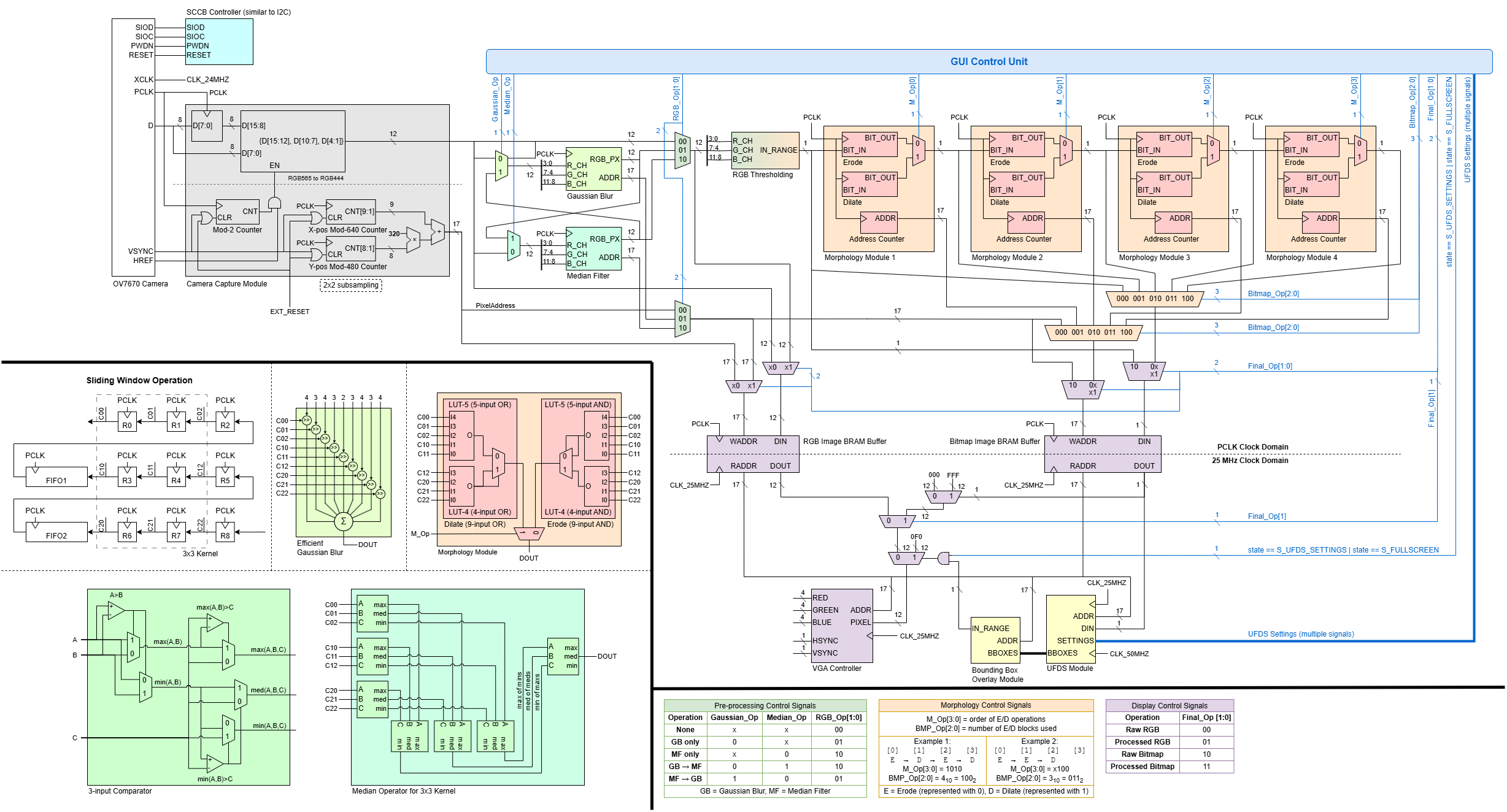
Servo PD Controller
Tracking is closed-loop at the pixel level: the centroid produced by UFDS becomes the measurement for a PID controller, and the controller output becomes the servo command. In Top, the PID is enabled only when at least one component is detected (comp_count != 0) and the system is in UFDS/fullscreen modes, which prevents the servos from hunting on noise during UI configuration. The setpoints are chosen as the center of the ROI (155 for x and 120 for y on a 310×240 grid), so “zero error” corresponds to the object being centered in the camera view.
The pan and tilt loops are implemented as separate instances of PID_Controller with fixed-point scaling implemented through bit shifts (KP_BITSHIFT_LEFT, KD_BITSHIFT_RIGHT) rather than floating point. Gains are exposed as small registers (pan_kp, pan_kd, tilt_kp, tilt_kd), and an integral limit clamps windup. The PID outputs are bounded to safe servo ranges (for example, tilt is constrained to SERVO_MIN=50_000 and SERVO_MAX=150_000) and then passed into Servo_Controller, which generates the actual PWM waveforms on servo_x_pwm and servo_y_pwm. A separate enable (servo_user_en from the UFDS settings UI) allows the user to toggle whether the physical rig tracks at all, which is important for safe demos.
Mechanical Design
The mechanical side is intentionally aligned to the control assumptions baked into the RTL. The servo setpoints are the ROI center and the UFDS centroid is measured in the ROI coordinate frame, so the pan axis is treated as “horizontal image x” and the tilt axis as “vertical image y”. That only behaves sensibly if the camera is mounted so that its optical axes are roughly orthogonal to the servo axes and the bracket does not introduce significant coupling. In practice, the mechanical mount is designed so that the camera’s field of view sweeps cleanly with pan/tilt and does not significantly translate relative to the rotation axes, which keeps centroid-based control stable.
The design also anticipates servo limits and dead zones. The RTL clamps the tilt range to avoid driving the bracket into mechanical hard-stops, and the PID enable logic prevents actuation when UFDS has no valid target. Together, the hardware control constraints and the mechanical constraints form a single system: the FPGA never assumes “infinite” actuation authority, and the rig never relies on software intervention to stay within safe motion ranges.
Conclusion
This project is essentially a full embedded vision system built in synchronous logic. The CV pipeline demonstrates how classical image processing can be expressed as windowed streaming operators; the UFDS engine demonstrates how a non-trivial data structure (union-find) can be implemented as a variable-latency FSM with explicit memory-backed state; and the GUI demonstrates that even “drag and drop” can be reduced to hit-testing, state updates, and deterministic raster overlays. The most valuable outcome for me was not the demo video itself, but the experience of making disparate FPGA concepts—BRAM timing, CDC, raster pipelines, and control loops—compose into a single coherent real-time system.